As a follow up to my prior article on Black-Scholes in PyTorch, I wanted to explore more complex applications of automatic differentiation. As I showed before, automatic differentiation can be used to calculate the sensitivities, or "greeks", of a stock option, even if we use monte carlo techniques to calculate option price. As it turns out, many exotic options can only be priced using monte carlo methods. Many exotic options are "path dependent", meaning their payoff depends not only on the final price of the underlying but also the behavior of the underlying throughout the time period. This often makes it impossible to use closed-form equations to calculate their price.

The traditional approach to value these options is to generate thousands of scenarios of stock prices and calculate the option payoff under each scenario. This is the essence of the monte carlo simulation. Often, to calculate option greeks, we re-run the monte carlo simulation several times with small differences in model inputs to see how the price changes. This process can be time-consuming when the number of inputs is large, or when the model is computationally intensive. Automatic differentiation may be able to provide more accurate sensitivities in less time than traditional methods.

In this article, I'll price five different exotic options contracts and use automatic differentiation to calculate the option greeks. I'll illustrate a few interesting scenarios from the thousands of monte carlo paths, and compare the sensitivity of the different options to the inputs of our simulation.

Creative financial engineering

Exotic options are amazing and creative. Chances are if you can imagine a bet you want to take on a stock there is a derivative contract for it. This is a short list of interesting contracts that we will price using the monte carlo scenarios.

Asian option: payoff is based on the daily arithmetic average underlying price over the entire time period, rather than the price on the expiration date.
Lookback option: payoff is based on the most optimal opportunity one might have had to exercise the option during the time period.
Barrier options: payoff is conditioned on the underlying security reaching (or failing to reach) a predefined threshold, called the barrier.
Cliquet option: this is a basket of forward-starting options that periodically settle and then reset over the time period.

Monte Carlo Scenarios

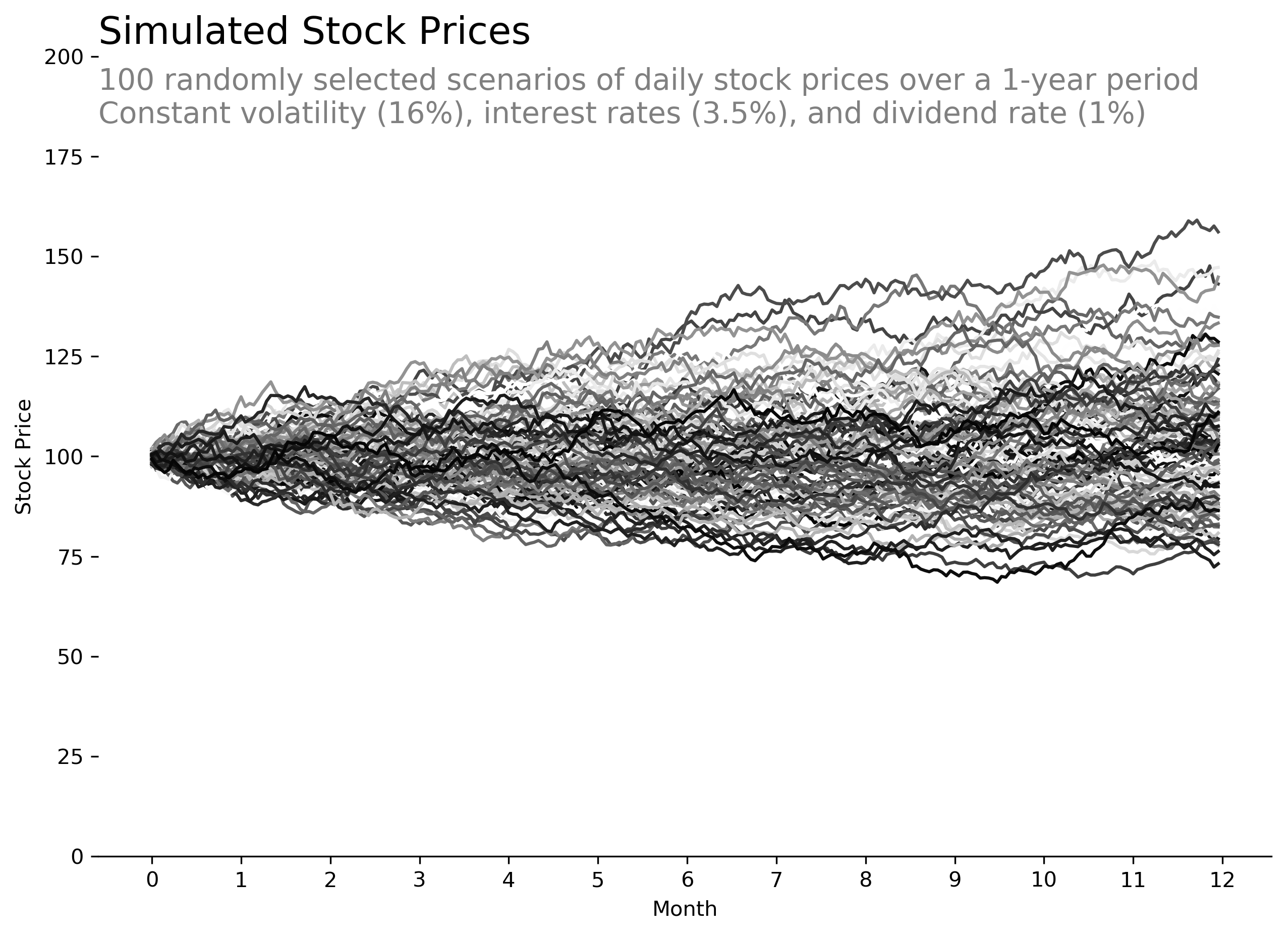
I'll use the same set of 1 million scenarios for each valuation to reduce the impact of random noise when we compare results. Each scenario will be comprised of 252 time steps (the approximate number of trading days in a given year.) As a result, we'll have a PyTorch tensor with size (1000000, 252). Each value in the tensor will be the total return for the stock on a given day for a given scenario.

I'll use the scenarios, which I'll call paths, to calculate a payoff tensor for each exotic option. The payoff tensor represents the cash flows generated from each scenario of our simulation. Because those cash flows happen at various times in the future, I'll discount them to today to calculate a present value. Then I'll calculate the average present value across all million scenarios in order to estimate the price of the option, which I'll call ov.

First, let's start by defining the variables that will be used to generate our scenarios. Then let's visualize 100 randomly generated stock paths to make sure things look reasonable.

# input tensors
stock = torch.tensor(100.0, requires_grad=True)
strike = torch.tensor(100.0, requires_grad=True)
vol = torch.tensor(0.16, requires_grad=True)
rate = torch.tensor(0.035, requires_grad=True)
dividend = torch.tensor(0.01, requires_grad=True)

# geometric brownian motion
torch.manual_seed(42)
scenarios = 1000000
step = 252

dW = vol * torch.randn(size=(scenarios, step)) / step**0.5
paths = (rate - dividend - vol*vol/2) / step + dW
paths = stock * torch.exp(torch.cumsum(paths, dim=1))

# discount rate per step
discount = -torch.cumsum(rate.repeat(step), dim=0) / step
discount = torch.exp(discount)

The Vanilla European option

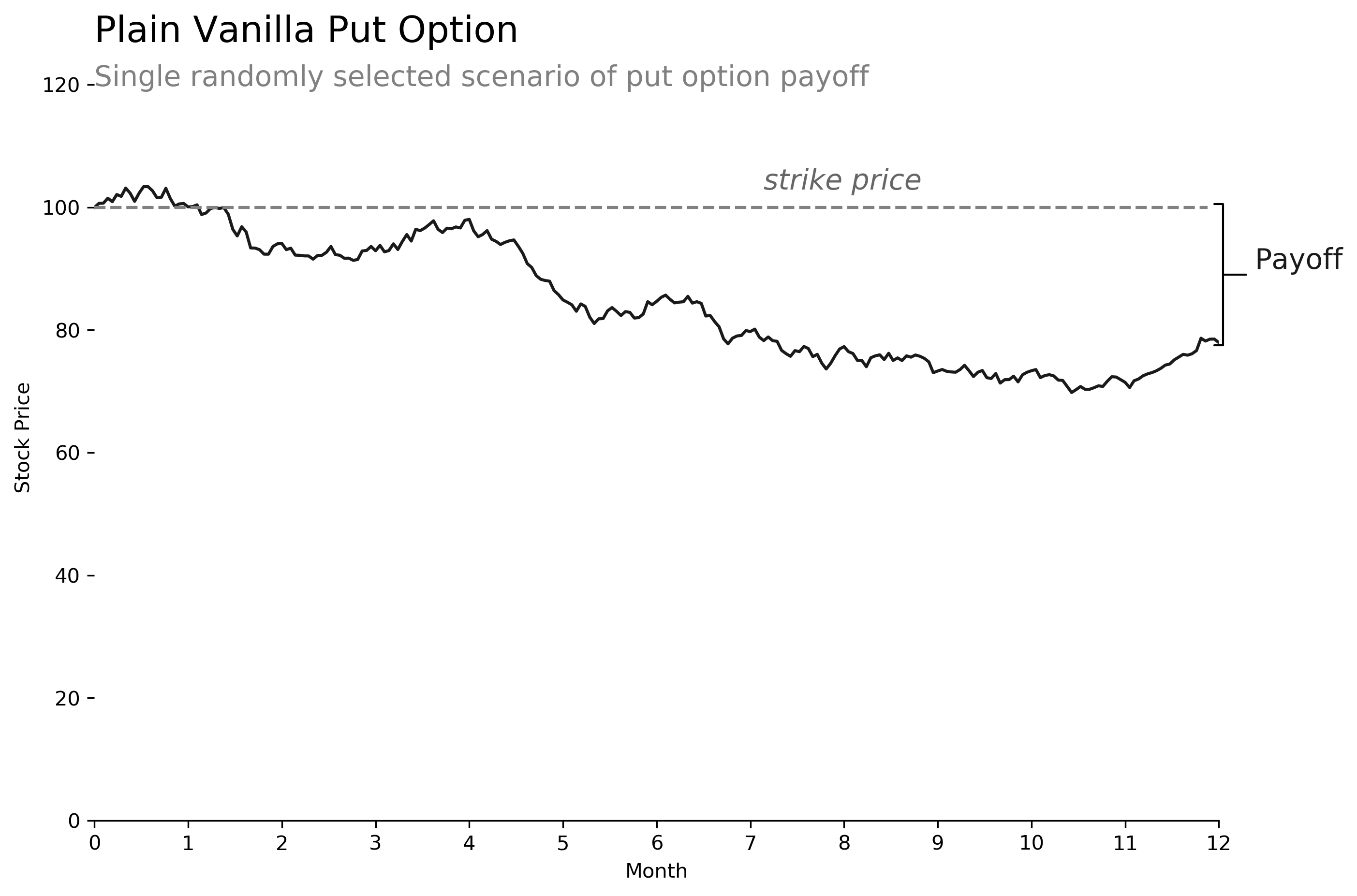
For the sake of comparison, we'll calculate the value of a standard European put option. This should be very close to the Black-Scholes value we calculated in the prior article. (Note that the prior article used 100,000 scenarios instead of 1 million, so the option prices are slightly different.) We'll also illustrate a single scenario to show how the option payoff is calculated.

# european put option payoff
payoff = torch.max(strike - paths[:,-1], torch.zeros(size=(scenarios,)))
ov = torch.mean(discount[-1] * payoff)

>>> print(ov)
5.0827

Asian option

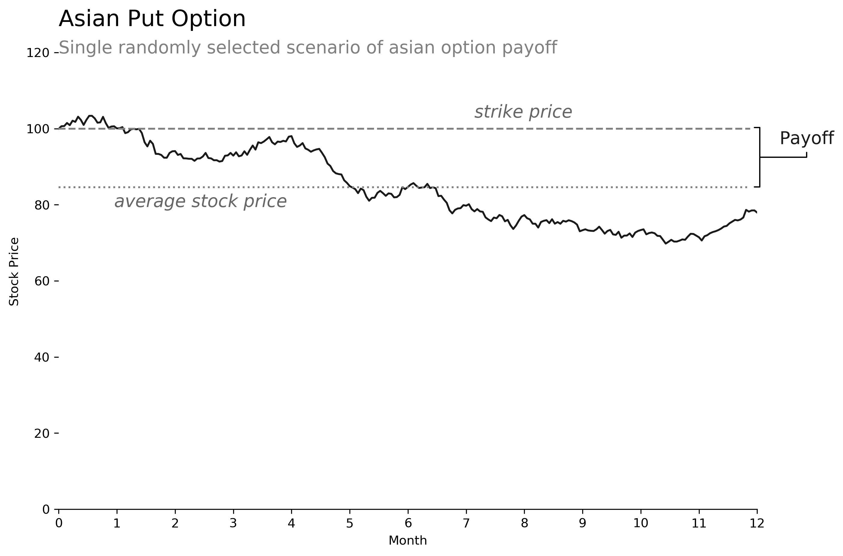
An asian option payoff is based on the daily arithmetic average of underlying price over the time period. This requires a simple change to our formula above. As we see, the price of this option is roughly 40% less than the standard European put option. Intuitively this makes sense, because the averaging mechanism makes it less likely for extreme option payoffs by the time we reach expiry. This is true for both call and put options.

# asian put option payoff
payoff = torch.max(strike - torch.mean(paths, dim=1), torch.zeros(size=(scenarios,)))
ov = torch.mean(discount[-1] * payoff)

>>> print(ov)
3.0117

Lookback option

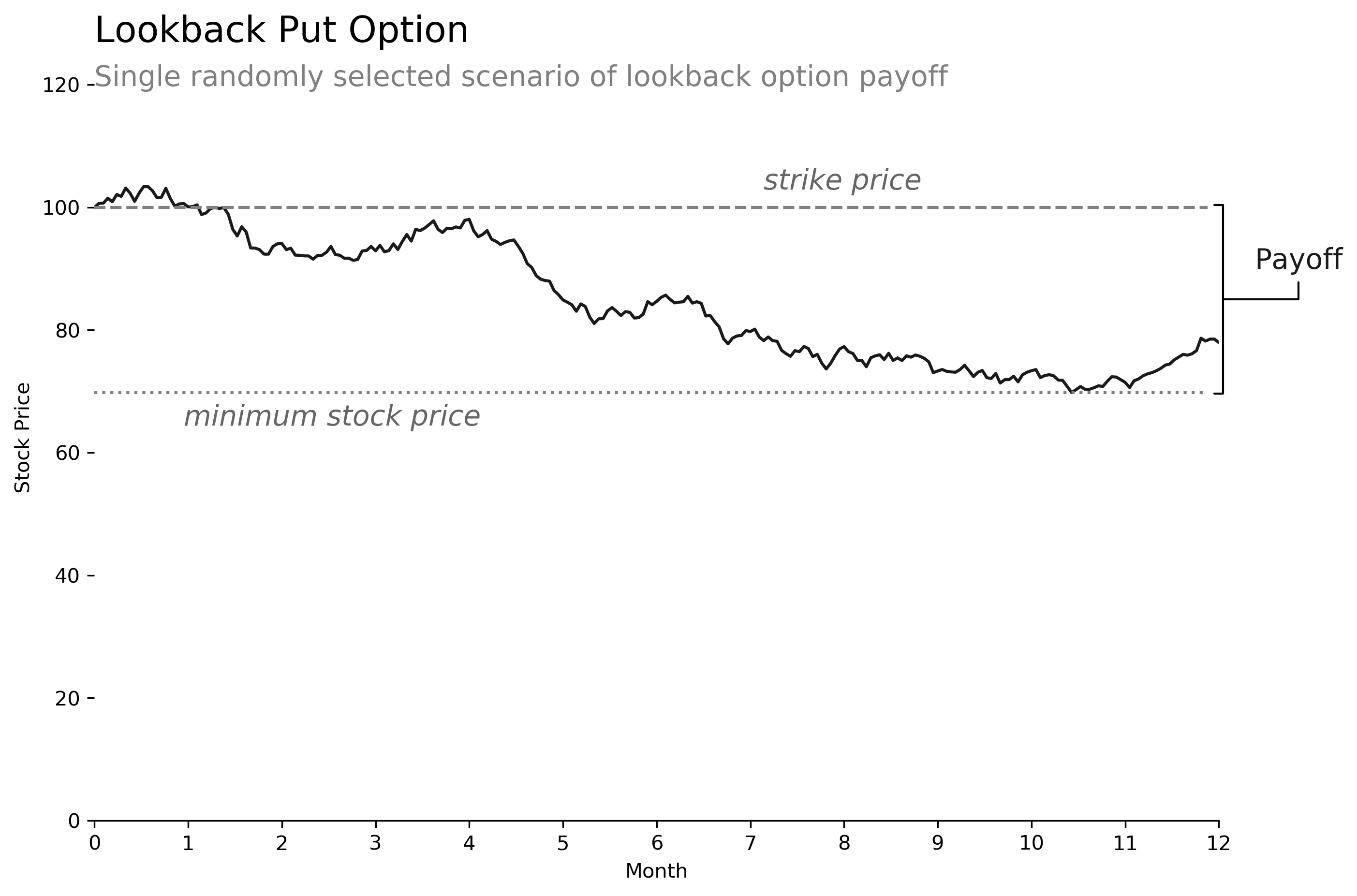
A lookback option payoff is equal to the optimal exercise value achieved at any point during the time period. In other words, the option owner is allowed to "look back" at the underlying price and choose the value that would result in the highest payoff.

For a lookback put option with a fixed strike of $100, the option holder will choose the minimum underlying price over the time period as the exercise price. In cases where the minimum is still higher than the strike, the option payoff will be zero, otherwise it will be the strike price minus the minimum value. Because the lookback put option is so advantageous, it often costs considerably more than a plain vanilla put option, as we see below.

# lookback put option payoff
payoff = torch.max(strike - torch.min(paths, dim=1)[0], torch.zeros(size=(scenarios,)))
ov = torch.mean(discount[-1] * payoff)

>>> print(ov)
10.2009

Barrier options

Barrier options, also called "knock-out" or "knock-in" options, have a secondary condition for exercise. In the case of a knock-out put option, if the underlying price falls below a certain barrier, then the option is invalidated and the payoff is zero. In the case of a knock-in put option, the underlying security must reach the barrier, or else the payoff is zero.

As expected, the option price for either barrier option is less than the price of a plain vanilla put option because of the more restrictive clause in the contract. It is also worth noting that the price of the knock-out option plus the price of the knock-in option equals the vanilla put option price. Intuitively, this makes sense, because the knock-in and knock-out options are like mirror images of one another. Owning both options would guarantee the exact same cash flows as the plain vanilla put option, which means the price should be the same too.

# barrier tensor
barrier = torch.tensor(80.0, requires_grad=True)

# determine if the option gets knocked out or knocked in
knockout = (paths > barrier).all(dim=1).type(torch.float32)
knockin = (paths > barrier).any(dim=1).type(torch.float32)

# knock-out put option payoff
payoff = torch.max(strike - paths[:,-1], torch.zeros(size=(scenarios,)))
knockout = torch.mean(discount[-1] * payoff * knockout)
knockin = torch.mean(discount[-1] * payoff * knockin)

>>> print(knockout, knockin)
2.4708, 2.6118

>>> print(knockout + knockin)
5.0827

Cliquet option

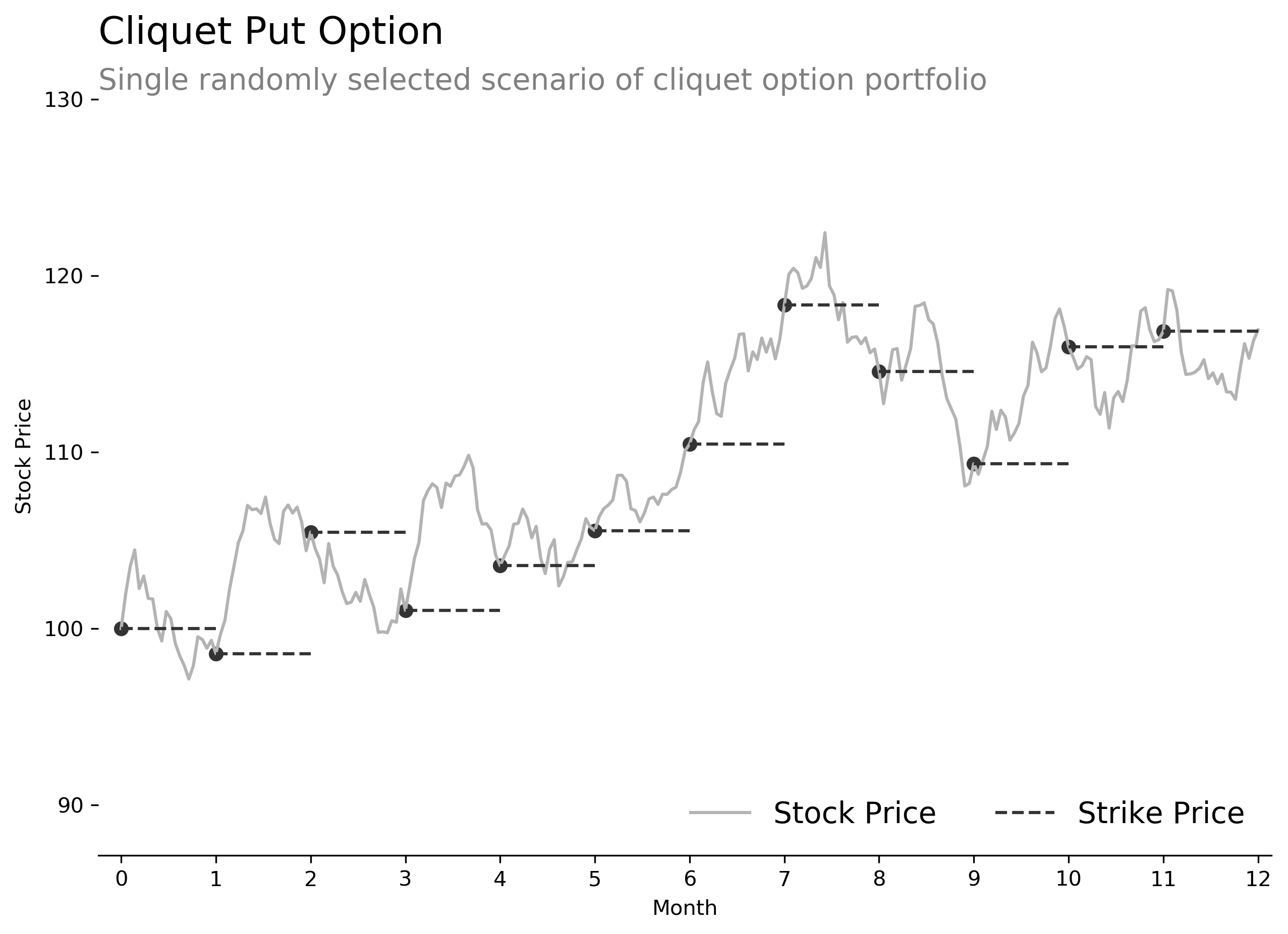
A cliquet option is a basket of forward-starting options that periodically settle and reset over the time period. For example, a monthly cliquet option over a one year time period is a portfolio of 12 forward-starting options - one for each month of the year. The starting strike price is fixed, in our case at $100, but at the end of each month, the prior option payoff is calculated and a new option is issued with a strike set equal to the current underlying price. In other words, a cliquet option is a way of paying for a portfolio of at-the-money options up front, without knowing what the future strike prices of the options will be.

The code for this option is slightly more complex. First, we identify the days that our options will settle and reset. For monthly put options, that will be every 21 days. Then we use the values of each simulated path on those days as our settlement and strike prices. The option payoffs for each month are equal to the prior strike minus the new strike. The periodic settlements are paid each month, so we discount them back to today's dollars to calculate a net present value. Finally, we average across all scenarios to estimate the option price.

Note that the price of a 1-month at-the-money put option with the same interest rate and volatility assumptions is 1.7369. Thus our cliquet option price of 20.7419 is roughly equal to $12 \times 1.7369 = 20.8430$ .

# determine the indices and values on the reset dates: every 21 days
strike_idx = np.arange(20, step, 21)
strike_val = paths[:, strike_idx]

# calculate the monthly stream of payoffs for each scenario
start = torch.cat([strike.repeat(scenarios, 1), strike_val[:,:-1]], dim=1)
payoff = torch.max(start - strike_val, torch.zeros_like(start))
ov = discount[strike_idx] * payoff
ov = ov.sum(dim=1).mean()

>>> print(ov)
20.7419

Comparison

The amazing thing about our simulations is that each option's greeks can be calculated using automatic differentiation. Because the option value is calculated from tensors whose gradients we are tracking, we simply call ov.backward() to tell PyTorch to propagate gradients backward, then call variable.grad for each of our inputs to calculate option greeks. I think it's incredible that despite the various idiosyncrasies of each option, it's possible to use the exact same automatic differentiation method to calculate option greeks. Now, let's compare option prices and greeks for our portfolio of exotic options.

                 Vanilla      Asian   Lookback  Knock_out   Knock_in    Cliquet
Option Value:     5.0827     3.0117    10.2009     2.4708     5.0926    20.7419
------------------------------------------------------------------------------
       Delta:    -0.4025    -0.4215    -0.8260    -0.2991    -0.1034    -0.2817
         Rho:   -45.3357   -23.8184   -49.8733   -32.3804   -12.9553   -48.7485
        Vega:    38.3756    22.2014    67.4165    21.6336    16.7419   137.1079
     Epsilon:    40.2530    20.8067    39.6724    29.9096    10.3434    37.5303
 Strike Sens:     0.4534     0.4517     0.9280     0.3238     0.1296     0.4861
------------------------------------------------------------------------------

There are several interesting comparisons to make among the different options.

We see muted greeks for the asian option. Overall it is less sensitive to all model inputs except stock price. This clearly reflects the averaging component of the payoff.
Next, we notice the lookback option vega is almost double the plain vanilla put option. This also makes sense: with the ability to choose the optimal value to exercise the option, we benefit significantly from volatile stocks that are likely to exhibit larger swings in price.
The knock-out and knock-in options are like two halves of the plain vanilla put option. The sum of both options together get us back to the plain vanilla option, both for price and for greeks.
The cliquet option represents a portfolio of 12 forward-starting options, and its price is roughly 12 times the price of a one month option. We notice that it is highly sensitive to volatility (the vega is nearly 4 times higher than the baseline!), which makes sense given its frequent resets throughout the year.

Overall, this was a fun exercise to use monte carlo simulation to explore some non-traditional financial derivatives. This is a viable technique for many financial valuation problems, and I look forward to exploring more applications in future articles.

Pricing Exotic Options in PyTorch