Riddler Card Collecting
Mar 1, 2019
Introduction
The Riddler Express this week asks us about collecting sets of cards. In particular, we're interested in collecting a complete set of 144 unique cards. We purchase one random card at a time for $5 each. How many purchases should we expect to make - and how much money should we expect to spend - in order to collect at least one of every card?
This problem can be approached in two ways: analytically, in which we develop and solve a formula to arrive at an exact answer, and via simulation, in which we model the card collecting process over a large number of trials in order to learn about the true distribution of results. Let's walk through each method below.
Analytical Solution
We can model this problem as a set of "states" and likelihoods of moving between those states. Each state tells us how many cards we've collected. For example, we begin in a state of "0 cards". Then we move to a state of "1 card" after we purchase our first one. It doesn't matter which card we get, because we know it will be unique. In order to transition to a state of "2 cards", we need to buy another pack and see a card we don't already own. Because there are 143 unique cards remaining out of the total set of 144, our odds of transitioning from "1 card" to "2 cards" are . On the other hand, our odds of staying in a state of "1 card" are , because there is a small chance that we receive the exact card we already have.
After this process continues for some time, we will arrive in a state of "143 cards" - we've collected all but one of the total cards, and we need one last card to complete our collection. Each new pack we purchase has a chance of giving us the card we're seeking, and a chance of remaining in a state of "143 cards".
We can define every possible state and all possible transition probabilities in a transition matrix. The transition matrix specifies the state we're currently in on the vertical axis, and the states we could move into on the horizontal axis. Here's one way to create this matrix in python.
import numpy as np

def transition_matrix(n_cards=144):
    """
    Create the transition matrix for any number of cards,
    where the default is 144 (taken from the problem).

    The matrix is all zeros except for the main diagonal and
    the upper diagonal, which are the probabilities of moving
    from one state to the next. All rows will sum to 1.0
    """
    # create the matrix, initialized with all zeros
    M = np.zeros(shape=(n_cards+1, n_cards+1), dtype=np.float64)

    # set the first off-diagonal elements, decreasing from 1 -> 0
    # this is the probability of finding a new card
    idx = np.diag_indices(n_cards)
    M[:-1, 1:][idx] = np.arange(n_cards, 0, -1) / n_cards

    # set the diagonal elements, increasing from 0 -> 1
    # this is the probability of finding a card we already have
    idx = np.diag_indices(n_cards+1)
    M[idx] = np.arange(n_cards+1) / n_cards

    # confirm we have a valid transition matrix where rows sum to 1.0
    assert M.sum(1).all() == 1.0
    return M
One nice feature of the transition_matrix function is that we can create matrices of any size, representing any number of unique cards. For example, we can generate the matrix for a set of five cards below.
>>> transition_matrix(5)
array([[0. , 1. , 0. , 0. , 0. , 0. ],
       [0. , 0.2, 0.8, 0. , 0. , 0. ],
       [0. , 0. , 0.4, 0.6, 0. , 0. ],
       [0. , 0. , 0. , 0.6, 0.4, 0. ],
       [0. , 0. , 0. , 0. , 0.8, 0.2],
       [0. , 0. , 0. , 0. , 0. , 1. ]])
Each row represents the starting state of owning a number of cards, starting with zero at the top and moving to five at the bottom. Each column represents the ending state, also from zero to five, left to right. For example, we see a probability of 100% that we move from a state of zero (first row) to a state of one (second column), where we see the number "1". We also see a probability of 20% that we move from a state of four cards (second-to-last row) to five cards (last column). Finally, if we start in a state of five cards (last row), we see that we're always going to end up in the same state. This is called an absorbing state because it is impossible for us to move anywhere else once we end up here.
Transition matrices like these have a fascinating property that lets us calculate the amount of time it takes to move from one state to another. We subtract the non-absorbing subset of our matrix, which is every row and column except for the last ones, from the identity matrix, take the inverse, and we have our answer! Here's what it looks like for our simplified five-card set.
>>> np.linalg.inv(np.eye(5) - transition_matrix(5)[:-1, :-1]).sum(1)
array([11.41666667, 10.41666667,  9.16666667,  7.5       ,  5.        ])
Each number in this array represents the time it takes to reach the absorbing state (where we have collected the entire set.) The array has the same length as the total number of cards. The first entry, 11.416, represents the time it takes to move from "0 cards" to "5 cards". The second entry, 10.416, represents the time it takes to move from "1 card" to "5 cards".
Now, to solve this week's riddler, all we have to do is apply the same logic to our full set of 144 cards. We're interested in the first entry in the array, which tells us how many cards we expect to see before we've collected every unique one.
>>> n_cards = 144
>>> np.linalg.inv(np.eye(n_cards) - transition_matrix(n_cards)[:-1, :-1]).sum(1)
array([799.27159218, 798.27159218, 797.26459918, 796.25051467, ... ])
We see that it takes an expected 799.27 random cards before we collect each of the 144 unique cards! At 5 dollars each, this means we have to spend roughly $3996 in order to collect the entire set.
Simulated Solution
Another way to solve this problem is to model the card collecting process and count the number of steps required to complete the set. However, because the process is random, every time we model it we will get a different answer. On the other hand, if we model the process a large number of times, say one million, then we would expect the average result to converge to the true result.
Here is the short python function that generates random trials. We run the function with a large number of trials to observe the distribution of results.
import numpy as np
from random import randint

def model(trials, n_cards=144, price=5):
    """
    Solve the riddler express via simulation: collecting cards, and
    counting the number of steps required to collect the entire set
    """
    for _ in range(trials):
        i, collected = 0, set()
        while len(collected) < n_cards:
            collected.add(randint(1, n_cards))
            i += 1
        yield i * price

trials = 1000000
results = np.array(list(model(trials)))

# print the average result
print(results.mean())
# 3995.78149
Good news! Our simulated result is very close to our analytical result above, at roughly $3996. The simulation also gives us information about the full distribution of results as well. For example, while it is theortically possible to collect 144 unique cards by drawing 144 unique cards in a row, the odds are extremely slim. What was the lowest cost from our simulation? What was the highest? This can all be seen by analyzing the results directly, or visualized as a density plot, which shows how likely it is that we would pay a certain amount to collect the full set of cards.
>>> results.min()
1795

>>> results.max()
13725
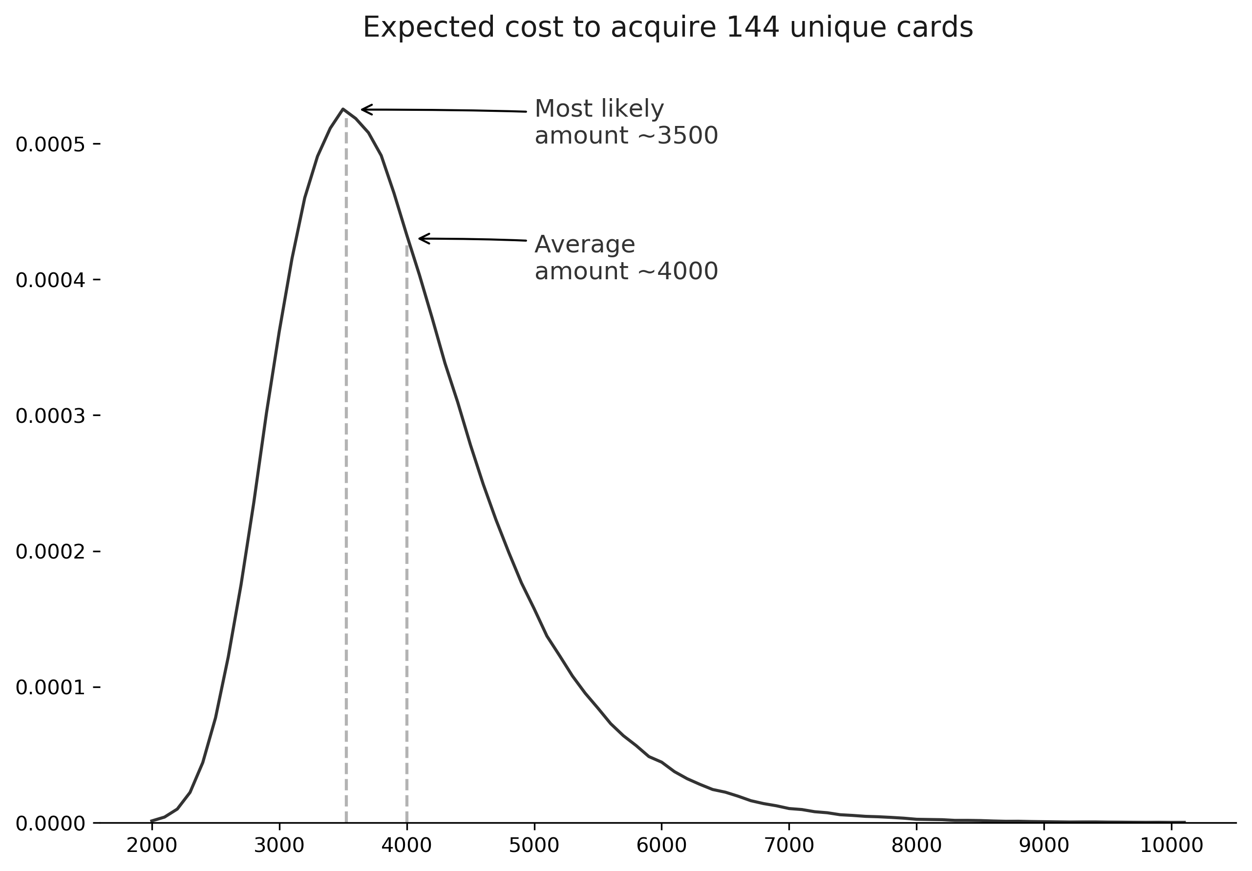
You'll notice in the chart that the most likely amount we'll pay to assemble the entire set is around 3500. However, the average amount we expect to pay is around 4000. Why are the numbers different? The average amount includes those tail scenarios where it takes us nearly 10,000 to collect the entire set, which moves it higher than the single most likely amount we would expect to pay. This is part of the reason why seeing the entire distribution, rather than just a single metric like the average, can be helpful in understanding the problem.